Introduction
With the increase in vehicle electrification and autonomy, electronic control units are now subject to rigorous functional safety standards such as ISO 26262. Functional safety is defined by ISO 26262 as “the absence of unreasonable risk due to hazards caused by malfunctioning behavior of electrical and electronic systems[1].”
Malfunctions are broadly grouped into two categories: random faults and systematic faults.
- Random faults occur unpredictably during lifetime of a hardware part and follow probability distributions[2]. Examples include component wear-out and bit flips in silicon devices due to thermal noise or energetic particles. Random faults can be further classified into transient faults (faults which resolve after a short time, such as a bit flip) or permanent faults which remain once present (such as a transistor damaged by a random voltage transient).
- Systematic faults are faults that are “manifested in a deterministic way that can only be prevented by applying process or design measures[3].” Examples include bad material batches, software bugs, and incorrect requirements. Systematic faults can also be introduced from software development tools; a compiler could produce anomalous code, or a test tool may generate incorrect test vectors or results.
The architecture of an electronic control unit establishes the likelihood for and ease of management of these two types of faults. Modern electronic control units can take advantage of several microcontroller architectures with different approaches to managing random and systematic faults. The main goals of any microcontroller architecture with respect to functional safety are:
- Manage random hardware failure in the microcontrollers
- Manage systematic failure in the hardware design
- Assist in managing systematic failure in the associated software
ECU Functional Safety Architectures
The two dominant controller architectures for electronic control units are:
- Multiple microcontrollers in separate packages
- A single microcontroller package
Multiple Microcontrollers in Separate Packages
Multiple-package architecture with diverse redundancy architecture utilizes two separate, physical microcontrollers working in concert to provide functionality and functional safety. The separate packages allow the selection of two different microcontrollers to provide diverse redundancy through different design and manufacturing.
This architecture can also support fail-operational behavior since a failure of one package may not prevent the other package from providing some degraded function. Since the microcontrollers are separate they can be powered by two independent power supplies to provide additional redundancy. The tradeoff is higher electronics complexity, typically larger footprint, and typically higher unit cost.
A Single Microcontroller Package
The single-package architecture is made possible by recent automotive microcontrollers that provide features such as lockstep cores (two redundant CPUs running the same code at the same clock rate with one delayed some clock phases with their results compared for consistency) and multiple cores (often with diverse design) in the same package.
This provides protection for many random hardware failure modes in a smaller hardware footprint which often has part cost benefits over multiple-package designs. Single-package architectures also generally require an external watchdog; increasingly these are being included in “smart” power supplies so there is no additional part count. However, the single package carries higher risk of dependent failures within the single package and is more limited in fail-operational use cases.
Comparison
The following section compares these two architectures in more detail
Robustness to Random Hardware Failures
Both diverse redundancy and modern lockstep-core + multiple core microcontrollers provide excellent protection against random hardware failures, both transient and permanent. Lockstep cores provide this checking with very little software overhead, while the diverse redundancy approach requires application software and communications protocols which can be a significant development effort.
Robustness to Systematic and Dependent Failures
Dependent failures are any failures that are not statistically independent. These are typically systematic faults even though they may have a probabilistic occurrence.
Hardware
Diverse redundancy is still the standard for minimizing dependent failures; two microcontrollers in separate packages with different design and manufacturers have very few opportunities for dependent failure. Independent packages are also less susceptible to the increasing threat of cybersecurity side-channel vulnerabilities such as timing-based attacks or privilege escalation.
Single-package architectures have greater opportunity for dependent failures due to manufacturing, common design of duplicated sub-components (for example, if lockstep cores are identical), and physical proximity.
Software
Lockstep cores cannot protect against systematic software fault concerns since the same software is run on both cores; Put another way: lockstep cores only cover hardware failure modes. This means that the processes for developing software on a lockstep core must still be performed to the highest applicable ASIL.
Most microcontrollers targeted for functional safety applications include additional CPU cores which are not lock-stepped in the same package to provide co-processing / checker capability. These cores are often of a different implementation architecture from the lockstep core, but care must be taken to ensure that there are no common sources of failure such as a common compiler.
For both single- and multi-package architectures that use co-processors or checker cores, the development of the software for each core should be performed by separate teams. Independent implementation, verification, and development tools such as compilers minimize the possibility for systematic errors.
Coexistence of Elements and ASIL Decomposition
Microcontrollers for both multiple- and single-package architectures are available with hardware-based memory protection units which can support partitioning of software.
A single-package design relying on memory protection hardware features requires the portions of software responsible for managing that memory protection to be developed to the highest ASIL.
Dual microcontroller designs, however, allow full decomposition of all software. For instance, it is possible to decompose all software two-micro system to ASIL B(D)+B(D), including for the operating system, because the two microcontrollers can provide redundant, independent coverage of the system safety functions.
Confidence in the use of software tools
Although the compilers for both microcontrollers in a separate-package architecture must be subject to software tool evaluation, the use of different compilers eliminates a source of systematic error since different compilers for different microarchitectures will not be subject to the same failure modes.
Since the software running on each core can be developed to a decomposed ASIL, savings can be realized in the tool qualification efforts to that decomposed ASIL.
Summary
Both the diverse-redundant multiple-package design and the single-package multiple-core designs can satisfy the functional safety demands of modern control units.
- Single-package architectures provide a simpler approach to managing random hardware failures, they require more analysis and development process diligence to manage systematic failures. The lower piece price for designs using single-package architectures makes this attractive for high-volume products even with the potential for higher development cost.
- Multiple-package architectures require more board-space cost but are more robust against dependent failures and can require less analysis due to more efficient ASIL Decomposition. The ability to decompose safety requirements and simpler analysis for dependent failures means development costs with multiple-package designs may be lower than single-package designs, offset by higher piece price; this architecture may be more suitable for low-volume projects.
| Multiple-Package Architecture | Single-Package Architecture | |
| Dependent Failure Robustness | Higher | Lower |
| Part Cost / Footprint | Larger | Smaller |
| Safety Analysis Effort | Lower | Higher |
| Software Implementation Effort | Higher | Lower |
| Tool qualification efforts | Lower per tool, but more tools | Higher per tool, fewer tools |
The OpenECU M560 and M580 vehicle controllers from Dana incorporate the Multiple-Package, diverse redundancy architecture, making them a compelling choice for low to medium volume projects with aggressive development schedules.
[1] ISO 26262-1:2018 Clause 3.67
[2] Adapted from ISO 26262-1:2018 Clause 3.118
[3] Adapted from ISO 26262-1:2018 Clause 3.165
Challenge:
Dana engaged with a large vehicle OEM to develop a custom ECU to be used on an autonomous vehicle demonstration fleet. All the OEM’s traditional suppliers refused to support the project due to the very aggressive timeframes. The ECU played a critical role in the overall vehicle positioning system and had to meet the following requirements:
- ISO 26262 ASIL-D
- Full redundant ASIL-D
- Fail-operational robustness to single-point failures (internal redundancy)
- Data transmission using 100BASE-T1 automotive ethernet (2-wire)
- Measurement and processing of high-resolution wheel position encoders
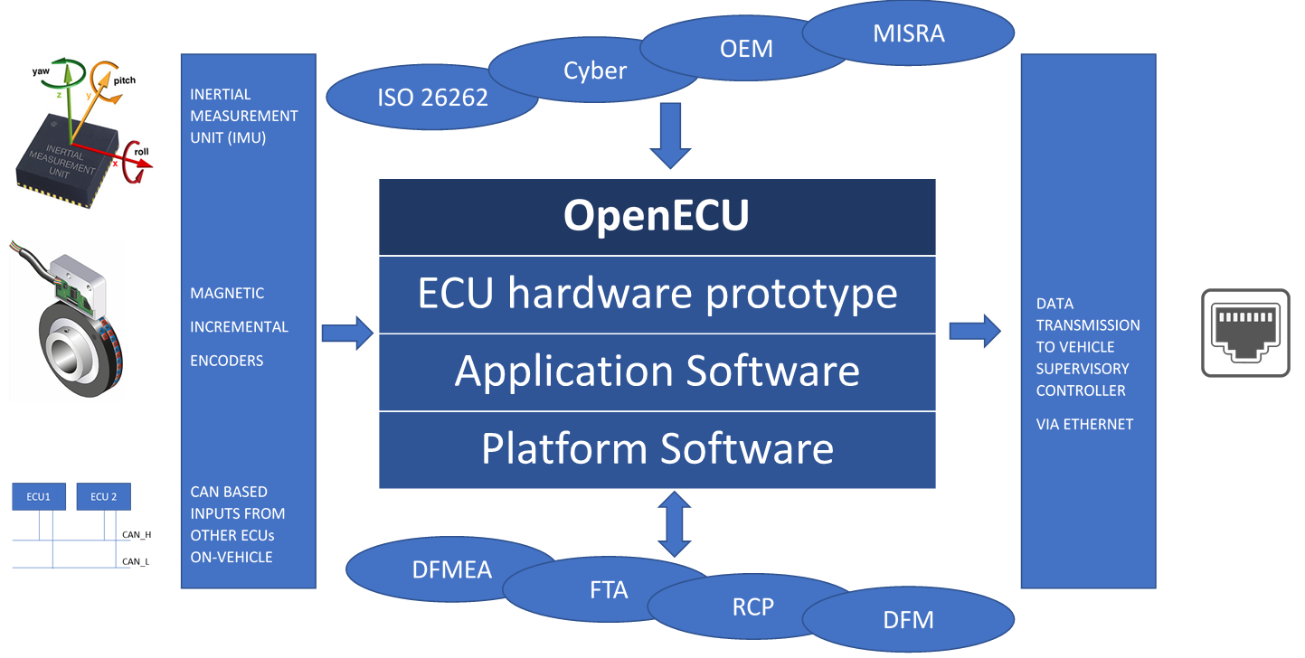
- 6-axis Inertial Measurement Unit (IMU) for vehicle attitude control
- High precision
- High stability
- Low thermal drift
- Data timestamping asynchronous sensor readings, based on the vehicle’s master clock module
- Compliance with the OEM’s internal processes and standards, including automotive cybersecurity requirements
Solution: Custom ECU Development
With a stringent timeframe of 9-10 months and limited requirements defined at the start, Dana compressed execution and delivery of the Custom ECU by paralleling hardware and software development. This was accomplished by highly leveraging the OpenECU platform for hardware and software development to meet:
- Functional safety (ISO 26262)
- Full redundant ASIL-D
- Customer cyber security requirements
- OEM ECU application requirements
This required full ECU hardware customization, OpenECU software customization, and ECU Application Software leveraging Dana’s Model Based Controls Development expertise using Simulink.
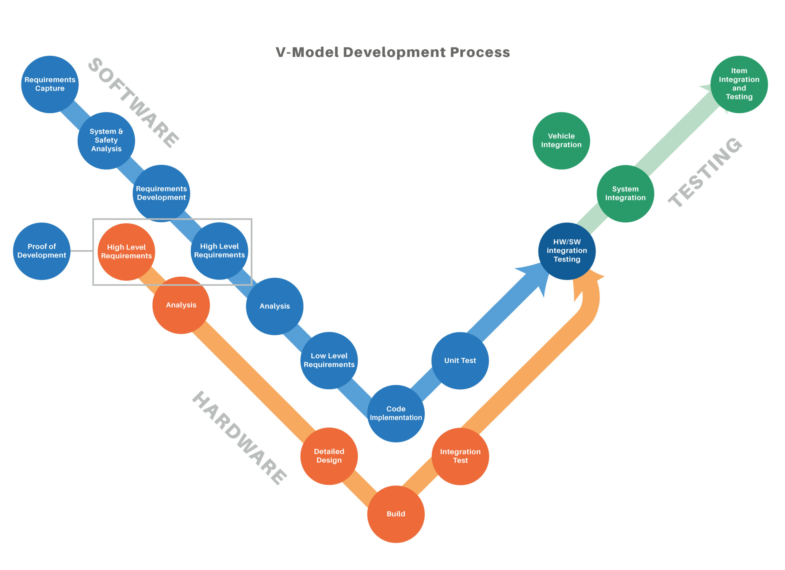
V-Model Process
Dana utilized the V-Model process while accommodating customer defined processes to develop the Custom Embedded Controller based on the OpenECU platform. Because requirements had not been established, Dana performed requirements solicitation for functional and safety requirements with a very large organization composed of a broad diversity of stakeholders. Dana’s extensive experience in requirements capture and analysis was leveraged in a multiple workshops involving all customer stakeholders to ensure transfer of design intent and information. Dana developed the specification for the module based on the following:
- System level safety analysis in conformance with ISO 26262
- Failure mode analysis (DFMEA)
- Fault tree (FTA) analysis
All unique system information and interfaces were taken into consideration to ensure that the hardware, underlying platform, and application software were designed to the elicited specification.
Hardware development
Based on the hardware requirements, Dana performed the following high-level tasks:
- Developed a conceptual CAD model to address mechanical and electronic packaging needs as well as heat transfer.
- Generated a new electrical design schematic using industry standard tools along with Dana’s own library of components.
- Developed a PCB layout following the schematic, while accounting for EMC requirements, heat dissipation, size, cost and functionality.
Dana’s hardware engineering team also used key techniques for hardware development to determine validation workflow early on and reduce the number of PCB spins. These include the following:
- Design for Excellence (DFX)
- Design for Manufacturing (DFM) and
- Design for DV
OpenECU software
Concurrently, software engineers at Dana developed the platform software incorporating the customization needed for compatibility with:
- Inertial sensors
- Magnetic incremental encoders
- Ethernet data transmission
- Cybersecurity
Specific OpenECU platform software builds covering all software and firmware requirements were developed and underwent static code analysis using PC-lint to ensure compliance with MISRA standards, OEM standards, and ISO26262 guidance.
Application software
The software architecture was decomposed to work on two separate CPUs within the same module following safety analysis, DAR and ASIL decomposition.
The control engineers were able to leverage the OpenECU rapid control prototyping (RCP) platform in Simulink to develop the main application software for one of the CPUs of the custom autonomous vehicle ECU. Redundant rationality diagnostics were contained in a separate CPU using a different application written in C language.
Since this was a high-integrity ECU solution, additional verification and validation (V&V) was also performed for model-based application software through Software-in-Loop (SIL) testing using VectorCAST environment. Dana also executed black box and DV testing of the new ECU in parallel to prototype testing of A-sample ECU’s in-vehicle, enabling the OEM to conduct integration testing early in the program.
A rapid turnaround of concept design to first prototype was ensured using close partners and key suppliers. Dana ensured that the custom hardware and software designs were integrated in an efficient manner while ensuring full traceability and compliance to all applicable standards.
Results and Impact
The project resulted in a custom ECU, a high-integrity sensor module, that met customer specific requirements and automotive standards. By leveraging the OpenECU rapid control prototyping platform along with expertise in design, development and manufacturing of ECUs, Dana was able to successfully deliver the prototype module to the customer in the required highly compressed timeframe. This was accomplished while incorporating customer driven processes, standards, and adhering to the highest level of functional safety requirements, critical in applications like autonomous vehicles.
Project Features
Keywords: Autonomous Vehicles, Custom ECU, Custom Embedded Controller, Functional Safety, ISO26262, Hardware design and manufacture, Custom software development, Rapid Controls Prototyping, Demonstration Fleet, Validation Testing
Introduction
Traditionally, replacing an OEM engine ECU or Engine Control Module (ECM) has almost always been out of the question. OEMs exercise proprietary rights to the hardware and software design used for engine control. This can often cause an undesirable delay, or even lead to a complete halt on advanced engine research programs or testing of new components on a base engine. Often, automotive organizations looking to modify ECU behavior face a big setback due to lack of access to engine controls.
Dana has developed a systematic approach to replace OEM ECUs (ECM) allowing full access to software and calibration, for prototypes, advanced technology development, demonstration fleets, or low to medium volume production programs. This is established with a combination of Dana’s engineering team expertise and the OpenECU family of rapid control prototyping ECUs and software suite. OpenECU is implemented to volume production standards and offers an accessible platform for custom configuration, adaptation, and further development. The goal is to provide a baseline engine control to customers to allow them to focus on what they do best.
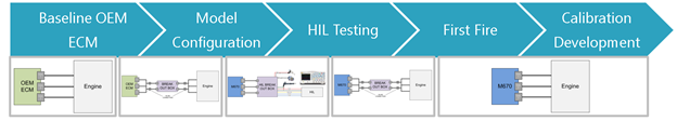 Figure 1: Dana’s approach for OEM ECU replacement
OEM ECU Replacement Process
1. Baseline the OEM ECU
The first step in this process is understanding the OEM ECU inputs and outputs, and mechanical configuration of the engine. Requirements capture related to characteristics of sensors and actuators is a critical step to confirm the compatibility of the engine system with the right OpenECU hardware. This is done using a customer questionnaire and preliminary review of available datasheets for different engine components. M670 is commonly used for engine control applications. M670 can also be customized to meet specific customer requirements.
In situations where data sheets for sensors are unavailable, and actuator characterization or trigger wheel patterns are not known, we use a bespoke break out box (BoB) and in-line connector setup allowing access to all the pins of the OEM ECU.
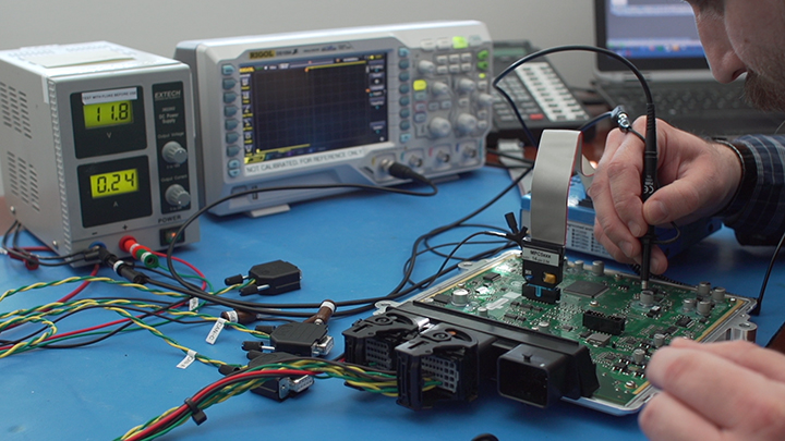
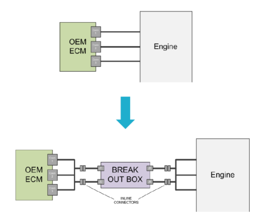 Figure 2: Setup for baselining the OEM ECU
This setup is then used to develop transfer functions for sensors, establish crank and cam patterns, and analyze output waveforms using dual instrumentation methods, oscilloscope measurements, etc. Important parameters are recorded to develop the baseline performance dataset. Some of the typical measurements made are:
- Injector timing and duration
- Number of injections
- Voltage and current recordings of actuators
- Fuel pressure for various speed and load conditions
A pin-out sheet to assign the available I/O to the relevant pins of the selected OpenECU module is drafted, which is the next step prior to model configuration and hardware-in-loop (HIL) testing.
2. Model configuration
Model-based control design (MBD) has gained significant momentum in the automotive industry to accelerate product development, while addressing the increased complexity of automotive systems, and reducing development time and costs. A rapid prototyping cycle is possible since MBD enables continuous simulation and verification of the control algorithm to allow early detection of errors, and the C-code is typically auto-generated which can then be deployed and tested on hardware.
At Dana, we have developed a model-based Generic Engine Control (GEC) strategy, which is accessible source code in the form of Simulink libraries (for both gasoline and diesel applications extendable to other fuel types such as LPG, CNG, etc.). These strategies are supported by documentation of the control architecture and software functional requirements for better understanding and knowledge transfer to the customer. The strategies can be used on OpenECU hardware to meet operating system needs. These strategies use floating point arithmetic and native Simulink blocks in the core of the application to allow for easier hardware target portability.
Within the model the crank, cam, and cylinder TDC configurations are appropriately set for the engine type. An application-defined sync logic based on crank and cam patterns is implemented to achieve engine sync. The OpenECU platform is designed in a way that allows software configurable waveforms for boosted/ non-boosted peak and hold injectors, saturating injectors and valves such as the fuel control valve, etc. that might require current controlled actuation.
The application is developed in a modular fashion and the required software modules can be integrated into the main model depending on the components involved in the application such as:
- Turbocharger
- Exhaust gas re-circulation (EGR)
- Variable valve timing (VVT)
The application incorporates a balance of first-principle physics-based modeling as well as 1D and 2D look-up maps, to characterize the underlying behaviors of different engine components. Commonly used functions are maintained in libraries and re-used to accelerate development and improve overall software quality. For production intent software, Dana focuses on the development of a modular architecture, which is essential since the software will go through inevitable expansion and refinement.
The model-based design approach lends itself to easy testing of the logic using simulation to prove the concept before integrating it with the main model. Further testing such as Model-in-Loop (MIL) and Software-in-Loop (SIL) testing can also be performed depending on the rigor required for the program.
The base calibration data available either from the customer or captured during the baselining process is integrated with the software before moving to the next step.
3. Hardware-in-Loop (HIL) testing
A one-click build system results in C-code generation: an S-record (s37) or Hex-record (hex) binary file along with an A2L file are generated. The A2L file contains all the information about measurement and calibration variables available in the control software and is typically utilized with industry standard calibration tools to communicate with the ECU via CCP.
The binary file is flashed on the OpenECU hardware, and HIL testing is performed with individual engine components to test basic functionality. This form of testing is made easier using calibratable overrides throughout the model. Crank and cam signals are setup using the HIL simulator, and the ability to achieve engine synchronization is verified first. OpenECU’s rapid control prototyping toolchain allows changes to be implemented and available on-target within a few minutes. This is of advantage for cases where there is interfacing with new components that might require quick software changes. After engine sync is achieved, injector firing and the waveform is verified along with actuation of other outputs such as spark, ETC, valves, etc.
This step also serves to identify any hardware changes that might be needed. Often a sensor might not function appropriately due to a different impedance than what is expected, and in cases like these OpenECU’s capability to be customized for specific system requirements becomes highly relevant. At Dana, this is referred to as an ECU ‘Option Control’. Some common changes in an option control are changing analog input pull resistance, changing low pass filter frequency of a digital input, changing pull-up source on analog and/or digital inputs, etc. Dana is also able to add completely new functionality to an existing OpenECU module depending on the specific needs of the customers such as 6-axis IMU addition to the OpenECU M670, piezoelectric pressure sensor addition to M670, etc.
After the option control exercise is completed and the available components are tested manually on the bench, the pin-out details are fixed, and the wire harness is developed by the customer.
4. First Fire
For this phase, a team from Dana typically arrives at a customer’s facility of choice. A dynamometer is used for the initial commissioning and calibration. The ECU is installed with the wire harness. One of the first steps is to perform signal and wiring checks for all sensors and actuators. If no issues are found, various key-on plausibility checks such as coolant temperature, battery voltage, etc. are performed. Crank and cam sync are established by motoring the engine without any combustion activity. This critical step ensures that engine sync is achievable which is necessary for enabling angular outputs/ actuators during normal operation.
At this point, the sensor transfer functions are also validated, and calibrated further as necessary. On the actuator side, angular outputs such as fuel control valve are verified against baseline data. Injector waveform and firing are confirmed by monitoring injector current and fuel rail pressure. If applicable, closed loop fuel rail pressure and cam phasing control are also tuned.
Once the operation of all the components is confirmed, the baseline calibration is verified. As a result, the engine is now able to operate with a new ECU.
5. Steady state calibration development
This step is intended for progress towards better engine operation with the new ECU. Traditional calibration refinement and verification activity in collaboration with the customer’s calibration engineers is performed. Steady state calibration is confirmed for various critical sections such as fueling, spark timing, target AFR, and cam phasing.
To further match OEM steady state performance, closed loop fueling, boost pressure control, and engine idling is tuned as well. Steady state operation across the engine’s nominal speed range is established.
A considerable amount of engine calibration is required to achieve the best performance from the engine control strategies, and once the initial steady state calibration is brought up to a pre-established customer expectation, a hand-off to the customer development team is performed. A training workshop is typically conducted at the end of the project to help the customer’s engineering team better understand the capabilities of OpenECU, along with new technology evaluations and understanding any future scope. Dana engineers train customer engineers while working alongside them to ensure the transfer of knowledge for full ownership.
CONCLUSION
OEM ECU replacement can be a tedious and complicated process. It can significantly affect advanced engine research programs, and customers looking to modify ECU behavior. With the OpenECU family of rapid control prototyping ECUs, and Dana’s expertise in system development and integration, you can accomplish ECU replacement seamlessly and in a short time frame.
Dana’s staged approach has been utilized in numerous engine programs. Dana can provide hands-on support with efforts ranging from commissioning and training on the OpenECU platform, through to providing full control software, hardware, and calibration, while being cost-effective and flexible.
To find out more about how Dana can help your organization replace an OEM ECU, develop a new prototype engine controller, or take your product from prototype to production, visit openecu.com or email info@openecu.com for more details.
Written by Mike Lepkowski & Ray Hyder
Option controls – Customizing OpenECU hardware for specific system requirements
Most systems require specific interfaces between controllers and sensors or actuators. While OpenECU has been designed to support a variety of sensors and actuators it can support an even larger variety of sensors through small changes to hardware in the ECU itself. Dana calls this modification an option control which uses one of our off-the-shelf OpenECU modules.
Option controls are best for customers developing prototype and low volume production systems where an existing OpenECU product meets most system needs but details of the interface between OpenECU and sensors/actuators require hardware changes. The most common option controls are changes to analog input circuits which allow OpenECU to exactly match the sensor interface as the sensor’s manufacturer requires.
Dana will work with you to define your requirements and come up with the best modifications to suit your application.
Which option control is needed for your application
Dana will work with you using our “Options and Variants” document that describes the default population of each pin on the module and the range of configurability that is available with an option control. Dana engineers will assess the compatibility of the customer’s I/O requirements with the default population of OpenECU and identify any areas where the default hardware configuration isn’t quite right for the system. Once those gaps are identified, Dana creates a custom option control which will configure OpenECU to be a perfect fit for the customer’s system needs/interfaces. Some examples of common changes in option controls:
- Changing analog input pull resistance
- Add/remove CAN termination
- Change the low pass filter frequency of a digital input
- Add/remove a freewheeling diode on a low side output
- Change the pull-up source voltage on analog and/or digital inputs
More advanced option controls
For customers with more specific needs, Dana may be able to add totally new functionality to an existing OpenECU. Some examples of specific functions added for past option controls:
- Piezoelectric pressure sensors were added to M670
- BLDC motor control was added to M250
- A 6-axis IMU was added to M670
- Current measurement was added to low side outputs on M220
- 4x H-bridge outputs were added to M670
Option control example
Recently on the M560, Dana worked with a customer to define their needs. The identified change was fairly small and made all the difference in making the M560 a perfect fit for the customer’s application. A digital input that was ranged for battery level 0-16V needed to be used as a 0-5V input. A change to the filter frequency was also identified as necessary to be compatible with the expected frequency of the sensor. Originally, the input had scaling for battery level inputs and was filtered for low-frequency inputs (25Hz). The scaling was changed to work with 0-5V PWM input and the filter frequency modified to work with 500Hz. This option control is now purchasable by the customer as the M560-00F.
What are you working on?
If you are not able to find an off-the-self controller solution to meet all your system’s needs Dana may be able to help with an option control for OpenECU.
The difficulty with diagnostics is in the definition.
- Do the diagnostics report simple wire harness shorts and opens checks?
- Do the diagnostics report ECU pin function checks and possible intermediate stuck at voltage checks?
- Do the diagnostics perform initial checks at power-on, or real-time and run-time checks of the internal ECU health and function?
- Are the diagnostics the complex rationality and long-term diagnostics of system (not just ECU) function related to regulatory compliance?
- Finally, are any of the diagnostics of functions associated with safety?
The answer is usually “yes to all the above”.
Basic Pin Diagnostics:
For most embedded control systems, the minimum price for entry is basic short circuit and open circuit diagnostics for all outputs. Inputs are more nuanced as the valid states for a typical switch input are “open circuit” and “short to battery” or “short to ground”. Fully diagnosable switch input circuits require switches which transition not between open and closed, but rather between two distinct closed states (distinct resistances to battery or ground) and are diagnosed with an analog voltage measurement. Measuring the analog voltage at the pin and comparing that to the expected voltage given the currently assumed system state is typically at the core of basic robust pin diagnostics. For more constrained systems or lower diagnostic intensity a simple digital monitor can often provide enough information, and in instances where frequency-based signals are expected, the ability to measure in the time domain may prove useful. The entire OpenECU product line has at least the basic pin diagnostics as a starting point.
Output Driver Diagnostics:
Output drivers have an idle state and an actively driven state (or potentially two actively driven states for H-Bridge outputs). The basic pin diagnostics needs to be cognizant of the possible valid pin states and the current commanded state. Do the diagnostics require detection of faults regardless of the commanded state? Do the diagnostics require detection of intermediate faults (not a short to battery/ground but an over current condition which could be caused by a short internal to an inductive load)? These diagnostics start with the pin state monitor (typically analog voltage for low speed circuits and possibly a digital input into a timer channel for frequency or PWM signals) and then diagnostic application code needs to be written to make sense of the pin state data. This diagnostic application code is usually tightly coupled to the control application, as the interpretation of the pin state data is highly dependent upon the expected state, which for outputs is determined by the control application. The output driver diagnostics provided by the OpenECU product line combined with the basic pin diagnostics enable the higher-level diagnostics to be constructed in the application.
Rationality Diagnostics:
Rationality diagnostics are not faults that drive signals out of their expected ranges, but more typically a set of input values that together do not match with a rationally expected physical system, e.g. the air/fuel ratio sensor reads lean mixture even at full fuel pulse duration and partial throttle. These diagnostic applications typically require substantial knowledge of the physics of the system under control, and usually need a large engineering effort to calibrate the thresholds between normal operation and faulted state. Quite often these applications require that data be stored from repeated operating cycles of the system.
Functional Safety Associated Diagnostics:
Functional safety associated diagnostics are more a mindset than a separate category of diagnostic type, involving diagnostics of faults/failures that do not directly cause an issue with a required function (input or output), but rather with a safety measure. If your system has functional safety associated controls, then an analysis is required where the ECU design is reviewed in light of the system safety goals, and the diagnostics must be reviewed to confirm that any fault that could violate the safety goals can be detected.
It is important to understand that even full-featured ECUs like the OpenECU M560, which have extensive diagnostic capabilities, will likely require application development to implement higher-level system diagnostic functions. Development of these system-level diagnostic functions for ECUs requires knowledge of the measurements and modes available on the ECU, in addition to the behaviors and details of the system under control. Dana’s extensive OpenECU documentation provides the necessary detail for systems engineers to develop these diagnostics.
Written by Gordan Jurasek, Director of Hardware Advanced Solutions, Dana
Evaluating the suitability of an OpenECU Electronic Control Unit (ECU) for use in your system as an embedded controller is best done in layers with the obvious and superficial screens done first to narrow the candidate pool to a limited quantity followed by the fine detailed requirements test on the narrower candidate pool. Many times, an off-the-shelf module will meet the requirements but for cases where customization is needed, OpenECU is designed to accommodate a wide range of options. The topics in this OpenECU evaluation series are:
- I/O
- Customization
- Mechanical Interfaces (vibration, thermal, mounting) & Usage Profiles of an Application
- Diagnostic Needs and Functional Safety
- Business Needs of the Program
- Design Verification Requirements
- Computational Needs of the Control Strategy
- Development Environment and Library Resources
How to Determine Which OpenECU is Suitable for My System: I/O
The first step in determining which OpenECU Electronic Control Unit (ECU) is most suitable is a simple matching of I/O capabilities to needs.
The tools I use daily to evaluate our ECUs for customer applications are the Pinout Templates for our line of OpenECUs. You can have a look at them on the Dana Downloads Page.

The information needed to properly evaluate a match between an application and an OpenECU is the following from the perspective of each ECU pin:
Analog sensor inputs:
- Does the sensor signal need a pull up to 5V or a pull down to ground in the ECU or does the sensor have a true voltage output which requires a high resistance input on the ECU?
- If it needs a resistance pull-up/down, what resistance value?
Digital switch inputs:
- Is the switch open/closed to ground or to battery?
Frequency/duty cycle inputs:
- Does the sensor signal need a pull up? If so, to 5V or to battery and what resistance value or maximum current?
- What is the maximum signal frequency?
Specialty inputs:
- Crankshaft/Camshaft, Wideband Oxygen sensor, thermocouples, knock, etc…
Outputs:
- Does the actuator require the ECU connect it to battery or to ground to turn the actuator on?
- What current does the actuator use when on?
- What is the maximum inrush current or stall current?
- Do the low side driven actuators need battery sourced from a high side switch output of the ECU?
- If the actuator requires a pulse width modulation (PWM) of the output:
- What frequency is the signal?
- What is the inductance of the actuator?
- Does the actuator require an H-bridge output?
- At what current?
- What frequency PWM? (or possibly DC only)
- Does the actuator require some specialty drive or waveform (i.e. 3-phase BLDC, Peak-and-Hold, Current mode control, other?)
- Do the outputs need to be synchronized with an input? (this can be simple pass thru trigger or complex synch like engine angle which is a derived clock from crankshaft and camshaft inputs)
Sensor supply and 5V reference:
- What is the sum of the sensor 5V power requirements in mA? (This number is typically 5-10mA per sensor, although some sensors do consume more.)
- Does your system require redundant 5V supplies?
Serial bus communication:
- What serial communication standards are used in your application? (CAN 2.0b, LIN, Ethernet, CAN-FD, J1939, SENT (SAE J2716), etc…)
- How many of each type are needed?
- Is wake-on-CAN required?
What are the power modes of the ECU:
- Connection to a switched battery supply which is only “hot on run”?
- Direct connection to system battery which is hot all the time with a separate “hot on run” signal used as ignition?
- Direct connection to system battery which is hot all the time with expectation that serial bus communication is used to wake the ECU?
- Sleep with periodic wake from internal RTC?
Written by Gordan Jurasek, Director of Hardware Advanced Solutions, Dana
As much as I would like (as an electrical engineer) to assume away any constraints presented by the physical world, there is no avoiding reality. Complicating matters is that some of the environmental conditions vary substantially with the operating modes. The operating modes, usage profile and conditions during each operating mode of the mounting location for the ECU must be collected. These consist of:
- Physical Interfaces:
- a. 3-D packaging space available.
- b. Assembly access for the ECU with its mounting brackets/fasteners.
- c. Wire harness access for connection and removal.
- Thermal Interfaces:
- a. Temperature minimum and maximum in that space during operation.
- b. Air flow thru the package space during operation.
- c. The expected power dissipation of the application. This might need to be estimated for each operating mode as the answers to items 2.a. and 2.b may differ substantially depending upon the operating mode.
- Vibration profile of the available mounting features.
- Ingress Protection:
- a. Water exposure conditions in the packaging space.
- b. Dust exposure conditions in the packaging space.
- c. Salt lifetime exposure expected.
- d. Chemical lifetime exposure expected.
The demands of the mounting location can then be compared to the capabilities of the candidate ECUs.
All of this can be quite a daunting task and may not be generally available at the start of a new program. Luckily for automotive applications there is a simple shorthand of a) in-cab, b) on-chassis (sprung), c) on-chassis (un-sprung), d) under-hood 105°C, and e) under-hood 125°C which have reasonably well accepted limits published in SAE and ISO standards and can be used for an early selection criterion and revisited when further application specific data is available as the program advances.
Note that operating modes are with respect to the overall system and not specifically the ECU. So, for a controller in an Electric Vehicle the modes might be Off, Charging and Run. For a pickup truck the Run mode might be further decomposed into Idle, Stop/Start traffic, Highway and Trailer Tow. The engine controller function might be nearly identical for Highway operation and Idle operation, but the air flow and thermal load is likely quite different. It is these differences which need to be captured to make a full mapping of the usage profiles and the mechanical and environmental interfaces.
A good example of a 105°C on-chassis rated ECU is the Dana M220 OpenECU.

Production Variants – Customizing OpenECU hardware for specific system requirements or cost optimization
Dana offers a wide variety of off the shelf modules that can fulfill the requirements of a broad range of applications. In some cases, there is a need to modify the off-the-shelf ECU to optimally work with specific sensors or actuators. In other cases, only a portion of the I/O is utilized to meet the requirements. In both cases, Dana offers the ability to customize existing off-the shelf ECUs to provide the most cost-effective solutions for production applications. We refer to these customized ECUs as production “variants”.
What is a production variant?
A production variant of an OpenECU module is very similar to an option control, except the circuit population changes are done at the factory during production. See the Part I of this Blog, “Option Controls” for information on how Pi develops option controls. As a short summary, Dana can provide development units with circuit changes implemented in our engineering lab to meet the needs of a customer’s system. A production variant is designed to be used as a production ECU, instead of just a development unit. The production aspect can allow for cost savings and would be PPAP capable.
How is a production variant developed?
There are two main avenues for how a variant OpenECU can be developed. The first, which is the usual case, is that they start out as an option control. When a customer has been using option control units finds that there will be a need for many more modified versions of the ECUs (possibly because they are going into production), Dana will work with them to create a variant. At that point, the development work for the customer’s system integration is done and the ECU modification needs to be released to our factory to produce the units directly. After that, ordering new ECUs with the modification can be streamlined.
The second avenue is directly developing a production variant. Dana will work with the customer to specify the variant directly when needs for low to mid volumes are apparent. Specific requirements and needs will be discussed and Dana will work with the customer to come up with the best solution for their system. After specification, Dana will create engineering samples to be tested on system to avoid “gotcha’s” (surprise changes based on unknown system elements) before releasing the variant to be produced in volume at the factory.
Production variant vs. Option control
Production variants are normally created when volumes above 50 are needed. Option controls are usually only development units from 1 to 50 pieces.
Production variants are made directly at the factory, instead of being modified at Dana. Since production variants are built at the factory they usually can be lower cost than modified off-the-shelf ECUs. Cost savings are from reduction in hand modification after the SMT process and potentially from removing compements not needed from the off-the-shelf version. Also, production variants can go through the PPAP process, while option controls cannot.
Variants will have some associated NRE for development, testing, and releasing of the variant part build documentation, but the costs are offset by lower per-unit cost vs. option controls, especially for low to mid volumes.
How it has been done before:
See case-study “Providing a new production EV supervisory controller with a customized M560”
An engine misfire can be defined as a combustion event where the air fuel mixture within a cylinder fails to ignite properly. The most common causes of misfire are:
- Incorrect air/fuel ratio, generally caused by a lean mixture
- Weak/missing spark due to wear of ignition system components
- Mechanical damage to the engine such as leaking gaskets, piston rings, etc, causing a loss in compression
Misfire has a number of undesirable effects, including
- Loss of power
- Increased fuel consumption
- Increased hydrocarbon emissions from the unburnt fuel
- Catalytic converter damage
Misfire and OBD-II
OBD-II regulations mandate the detection of misfire on all passenger vehicles. In most applications, the Engine Control Module keeps a count of the number of misfire events that occur over a moving window of engine revolutions. If the misfire count exceeds a threshold, a diagnostic trouble code is set.
Misfire Detection Using OpenECU
There are several ways to detect misfire. In this post, we will discuss misfire detection using the crankshaft position sensor. During a normal combustion event, the piston speed is lowest at top dead center on the compression stroke, and is the highest with the piston moving downwards during the power stroke. The average engine speed for a single engine revolution would lie in between the lowest and the highest instantaneous values. The difference between the lowest and highest engine speeds is significant enough that any deviation from the values expected during normal combustion can be used to detect a misfire event. If misfire occurs, the crank speed during the power stroke will be significantly lower as there is no downward force being applied on the piston head from combustion of the air fuel mixture. Figure 1 shows how the variation of instantaneous engine speed with crank angle for normal combustion and misfire conditions.
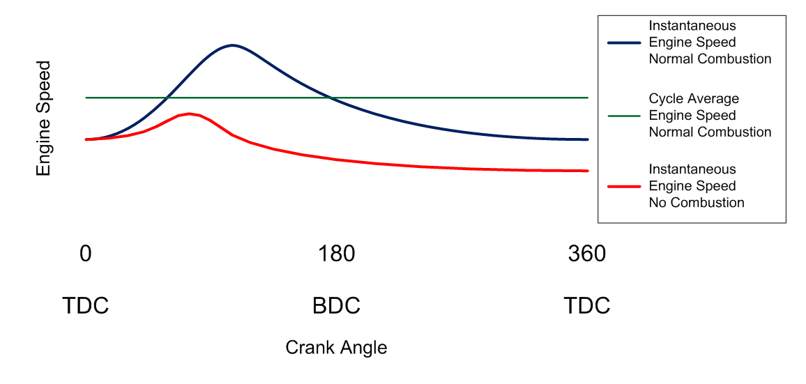
Figure 1 – Instantaneous engine speeds vs crank angle for normal combustion and misfire
The OpenECU Simulink blockset provides an easy way to calculate the engine speed during specific portions of the engine cycle using the crankshaft position sensor. In the example shown in Figure 2, each instance of the Engine Speed block is used to calculate the average engine speed over a different portion of the engine cycle. The first block gives the average engine speed over 720 degrees of crank rotation. The second block calculates the “post-TDC” or highest crank speed and the third calculates the “pre-TDC” or slowest crank speed during the engine cycle. The tooth range is calibratable, which means that it can be easily adjusted in real-time to account for varying operating conditions, such as a change in the spark timing, which can affect the location of the fastest crank speed relative to the TDC of the cylinder.
The tooth ranges can be specified relative to the TDC of each cylinder, or relative to the missing tooth region of the crankshaft position sensor pickup wheel. Each cylinder will have its own pair of blocks to detect the maximum and minimum crank speeds. The speeds calculated by the OpenECU blocks can then be compared and a misfire event can be detected if the separation between the two indicates that the crankshaft did not accelerate during the power stroke.
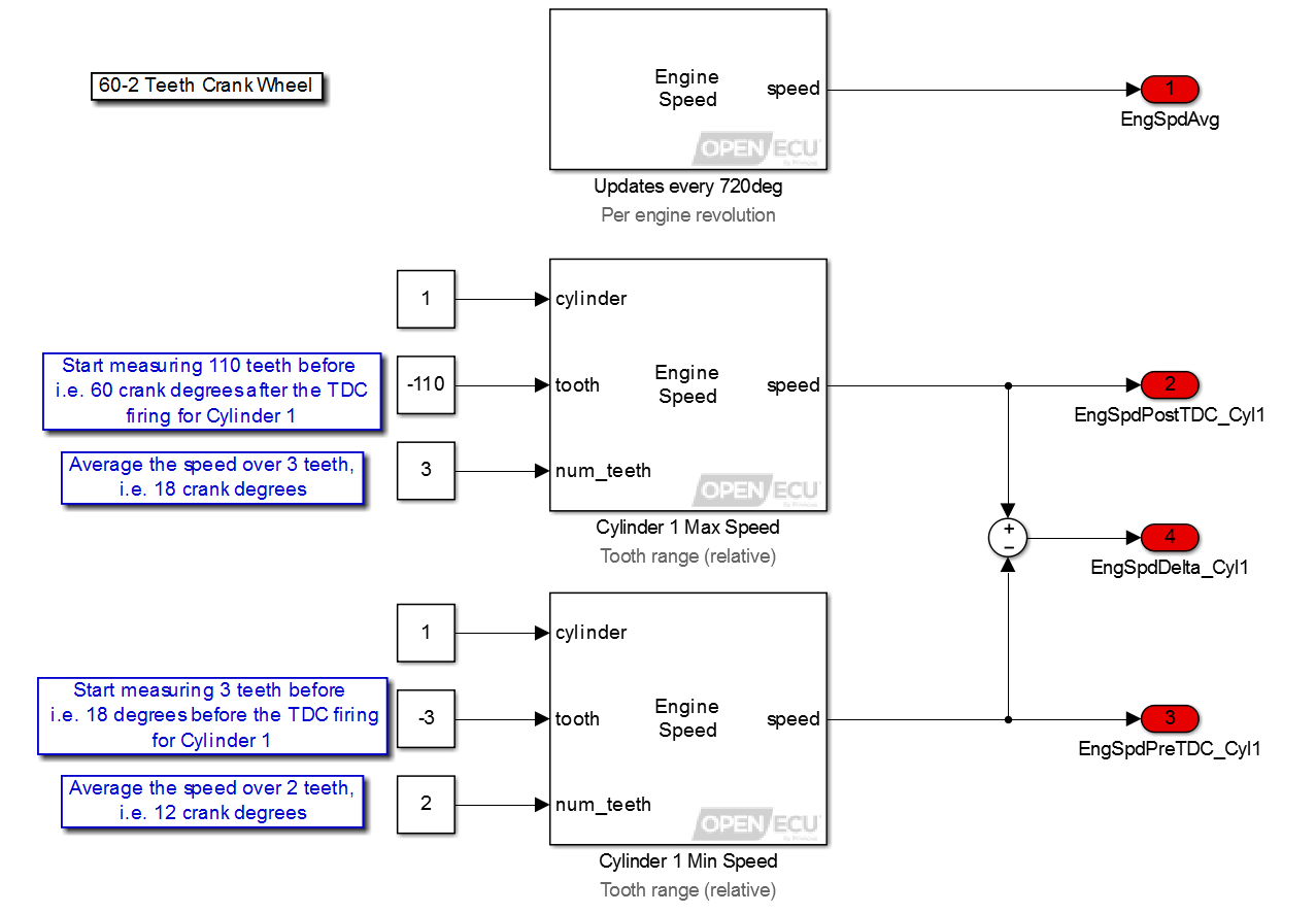
Figure 2 – Example implementation of TDC relative engine speed measurement with OpenECU
The figure below shows the pre and post TDC engine speeds when misfire events are induced on a single cylinder engine using an ignition cut. The reduced difference between the pre and post TDC engine speeds clearly shows the misfire events.

Figure 3 – Pre and Post TDC engine speeds during normal combustion and misfire
 Accessibility