This article provides an overview of the hardware and software architecture of a sinusoidal field oriented controller for a brushless DC motor (BLDC).  Brushless DC motors are becoming much more common in automotive applications due to their improvements in performance, efficiency, and reliability over brushed motors.

A brushless motor has to be commutated electronically, meaning that power must be applied to each of the 3 phase windings at just the right time as the rotor spins.  This requires an inverter which is capable of controlling the voltage at each motor phase.  The inverter is driven by 6 PWM outputs from the microcontroller, controlling whether each motor phase is connected to power or ground.  In order to determine the correct PWM states, the controller needs to know the rotor position (angle).  This can either be measured with a sensor, or it can be estimated from current and/or voltage feedback from the inverter.  For field oriented control, current feedback is required regardless of whether there is a rotor position sensor.

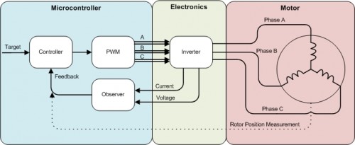
The diagram below shows the major components of the BLDC control system.

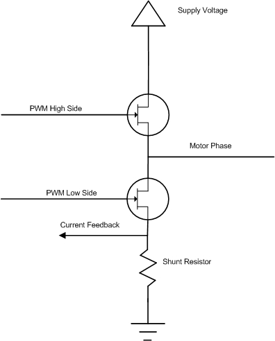
The inverter controls each motor phase voltage with a pair of FET’s which can apply either power or ground.  The PWM outputs from the microcontroller are paired together such that one controls the high side FET and the other controls the low side FET.  The PWM pairs are operated together in a complementary switching scheme, where they are never both on at the same time.  The phase current can be measured through a shunt resistor on the ground side of the inverter circuit.  In this setup, current flows through the shunt resistor when the low-side FET is turned on.  The diagram below shows an example circuit for 1 leg of the inverter.  This circuit is repeated for the other 2 motor phases.

There are many micro-controllers designed specifically for motor control which may have some or all of the following features:

The PWM outputs can be paired together to do complementary switching.  Since each motor phase is connected to 2 FET’s, they must be controlled as a pair.  Both FET’s must never be on at the same time; when one is on, the other must be off.

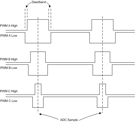
The PWM pairs have a configurable deadband between the complementary switch states. The deadband is a time delay between turning one FET off and turning the other on.  This prevents current shoot-through on the FET’s by preventing any overlap where both FET’s could be on simultaneously.

The PWM clocks can be synchronized with each other and center-aligned.  For a FOC system, the phase current is typically required on at least 2 of the 3 motor phases, and is measured through a shunt resistor on the ground side of the inverter circuit.  Since current only flows through the shunt resistor when the low-side FET is on, the PWM’s need to be aligned so that all of the current measurements can be sampled at the same time.

The ADC conversions can be triggered by the PWM clock.  This allows the feedback signals to be sampled exactly when current is flowing through the shunt resistors.

The diagram below shows an example of the complementary, center-aligned PWM signals which would drive the inverter.

The control algorithm transforms the motor phase currents to the reference frame of the rotor.  This transformation allows the sinusoidal phase currents to be controlled as DC quantities.  The two axes in this coordinate system are the direct axis, which is aligned with the rotor and the quadrature axis, which is perpendicular to the rotor.  The current vector of each axis is controlled independently, which allows the angle between the resultant vector and the rotor to also be controlled.  The q-axis controls the motor torque, the d-axis controls the motor flux linkage.  Maximum torque occurs when the resultant current vector is aligned with the quadrature axis (ie. Id = 0).

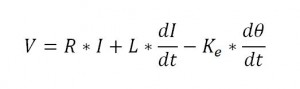
Since this whole control scheme is based on the rotor frame of reference, the rotor position estimator is the key component and it must be accurate.  One method of estimating the position is to use a back-emf observer.  As the motor speed increases, it creates a back-emf which produces a current that opposes that driven by the inverter.  A simple model of the motor can be implemented based on this equation.

 

In the next part in the series we will more closely investigate how to estimate the rotor position with this equation.

 

CANopen is a CAN-based communication protocol. It comprises higher-layer protocols and profile specifications to exchange data between multiple devices on a network. Today it is used in various applications, such as medical equipment, off-road vehicles, maritime electronics, railway applications, and building automation.

OpenECU provides a reference design containing six blocks to implement a CANopen communication network. These blocks are used to configure the CAN bus, monitor CAN bus status, transmit, and receive CAN messages. The CANopen reference design is built upon the OpenECU Simulink blockset.

Communication

CANopen devices use several types of messages for communication, such as, PDO, NMT, SYNC and EMCY messages. Despite the differences at the application level, the standard CAN message format is always the fundamental structure for exchanging information. This enables OpenECU to use its existing CAN blocks to act as a master CANopen device and communicate with CANopen slave devices.

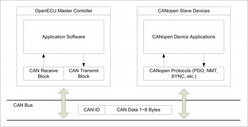
Typical CANopen System

The reference design model is used as an example to show how OpenECU can be used to realize communication and control of CANopen devices. This model has been validated in a motor control system which has a CANopen compliant inverter controller. OpenECU serves as the master controller and sends commands via CAN to the inverter, which acts as a CANopen slave, and provides feedback to the master. This configuration may be found in a hybrid or electric vehicle utilizing an inverter that uses the CANopen protocol.

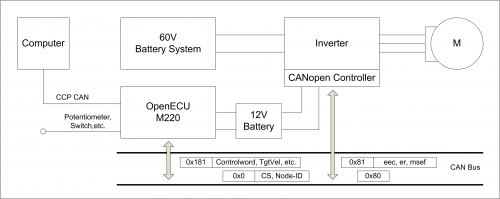
Example 1: PDO

Process data objects (PDOs) are used in CANopen for broadcasting high-priority control and status information.  For example, the master OpenECU controller uses PDOs to send motor speed mode commands to the slave the motor controller.  The slave motor controller in turn uses PDOs to feedback the actual motor status. A PDO consists of a single CAN frame and provides up to 8 byte of application data. The PDO objects need to belong to the CANopen object dictionary and both devices must have the same configuration.

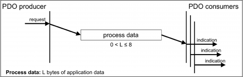
The reference design model sends and receives process data using OpenECU CAN blocks. Note that OpenECU CAN blocks use the Motorola byte order and byte reversal block may need to be applied.

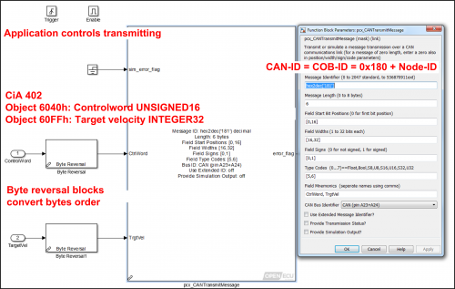
Example 2: NMT

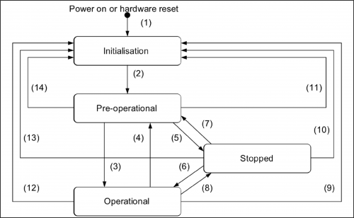
All CANopen devices must support the CANopen network management (NMT) state machine. The NMT state machine controls the communication behavior of a CANopen device. The CANopen NMT state machine consists of an Initialization state, a Pre-operational state, an Operational state, and a Stopped state. The NMT protocol is transmitted by the active NMT master in a CANopen network. The reception of the NMT protocol forces the CANopen device to transition to the commanded NMT state. The NMT protocol uses a single CAN frame with a data length of 2 bytes. It uses the CAN-Identifier 0x00, which is the highest priority CAN-ID in a CAN-based system. In the CANopen compliant motor control system, OpenECU as a master device manages network states through a state machine built in the reference model. The NMT command specifier is sent to the slave motor controller through the OpenECU CAN transmit block.

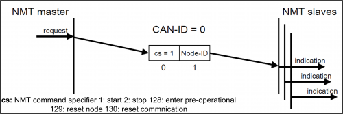
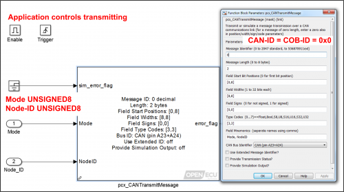
Similar to the PDO protocol, an OpenECU CAN transmit block can be used to implement the NMT protocol as well. Instead of putting process data on CAN message, the command specifier and Node-ID need to be specified as the CAN message data.

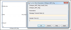
In the reference design model, a masked NMT block is provided from the CANopen library. It gives the interface to enable message transmission, change modes, specify the node ID of the slave device being commanded, and set the node ID, and the rate at which to transmit the message.

CAN DBC Support

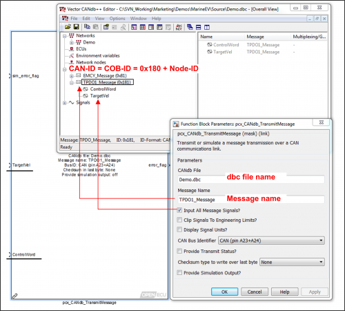
OpenECU also provides CAN blocks that can use a .dbc file to specify the message ID’s and content instead of explicitly defining the message structure of each PDO message. The principle is the same, but these blocks provide access to the information using the textual names assigned in the database, making the model easier to create and maintain.

CANopen Communication State Management

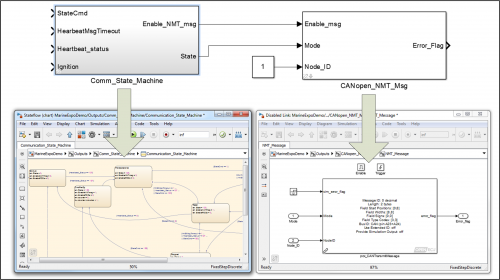
In addition to the CAN blocks used to transmit or receive messages from CANopen slave devices, a communications state manager is required by the CANopen protocol. The reference design model provides a state machine that determines the NMT state which is required by all CANopen devices.

As shown in the figure below the Stateflow chart on the left controls network states according to the requirements of the CiA 301.  While the the right side is implementing NMT protocol to transmit NMT data to slave device (Node-ID = 1) with OpenECU CAN block. Another example is application software calculates the target speed velocity and send to slave devices by PDO protocol.

Summary

OpenECU Simulink CAN blockset can implement several CANopen communication protocols without much effort. Pi provides a validated reference design model to demonstrate the methods. More complicated functions, e.g. network management, devices control and diagnostics, etc. can be implemented at application software level using Simulink blocks.

For more information on the CANopen standard please go to https://www.can-cia.org/can-knowledge/canopen/canopen/

By using digital communication, many sources of inaccuracies are eliminated as compared with traditional analog sensors, such as wiring resistance, circuit component tolerances, and A/D conversion gain and non-linearity errors.  Furthermore, more data can be placed on a single wire thus co-located such as manifold air flow and ambient air temperature sensors can use a single wire, thus saving on wiring harness costs.

One method of communication that is gaining popularity within engine sensors is SENT, also known as SAE J2716.  SENT stands for Single Edge Nibble Transmission protocol.  SENT uses the time between consecutive falling edges of a digital signal to encode a single nibble (4 bits) of data, where the longest time between falling edges represents binary 1111 (hex 0xF), and the shortest time between falling edges represents zero.

By encoding the nibbles using time, this allows for a high rate of data transmission at a lower cost than traditional serial communication.

 

Decoding a SENT signal

SENT messages typically have six data nibbles, allowing 24-bits of information to be transmitted per message.  It is common to have two 12-bit signals encoded in each message.  For example, an atmospheric temperature and pressure sensor may send the temperature in the first 3 nibbles, and the pressure in the second three nibbles.  The 24-bit message will then need to be split apart into the two signals using bitwise arithmetic.

In addition to the 6 data nibbles, messages contain a synchronization pulse, one nibble for status and communication information, and one nibble for CRC error detection.  The synchronization pulse is used by the receiver to calculate the exact bit-timing of the sender, thus making the system tolerant to small clock frequency differences between the sender and receiver.

 

SENT communication with OpenECU

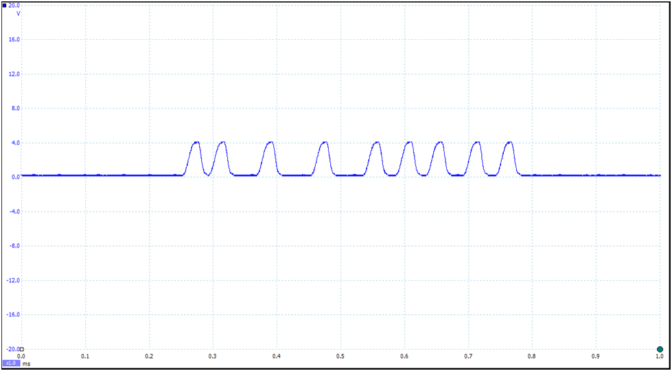
To show how SENT sensors are handled with OpenECU, we will use a throttle position sensor from a modern production engine.  Our sensor uses all 24 data bits of the SENT message to encode the throttle position, and communicates with a nominal communication tick duration of 3.4 microseconds.  A typical message waveform from our throttle position sensor is shown in the following oscilloscope capture:

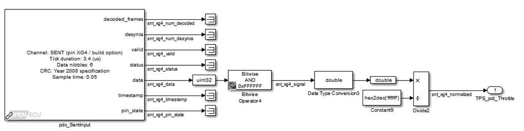
The OpenECU Blockset for M670 contains a SENT input block which handles all of the decoding of the SENT messages, including CRC checking and synchronization.  In our example, we extract the 24-bits of signal information, and convert the signal to a 0.0 – 1.0 number to represent throttle fraction:

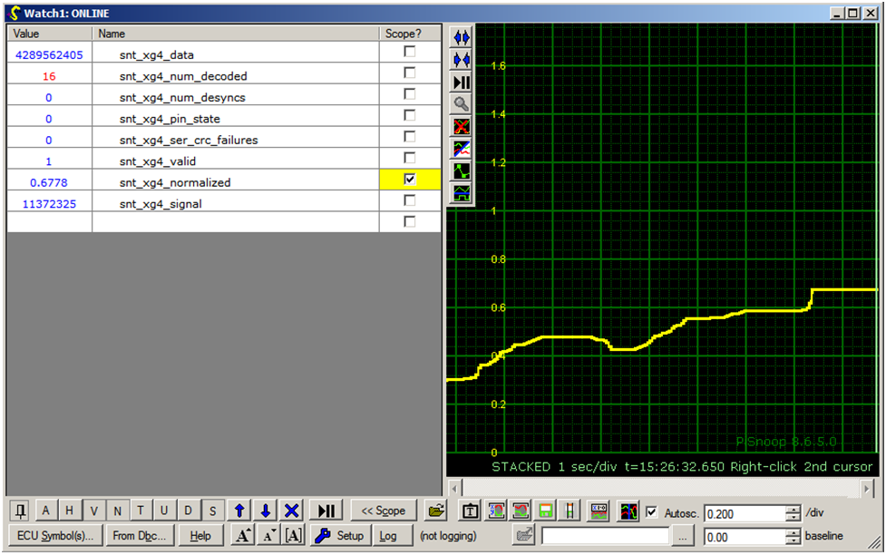
After building the model for the M670 and flashing the generated software onto an M670 ECU, the throttle position sensor could be easily viewed using a standard calibration tool.  A signal trace showing the throttle position using OpenECU Calibrator can be seen below:

Further information on SENT, can be obtained through SAE in the J2716 standard document.  A brief overview can be found on Wikipedia.

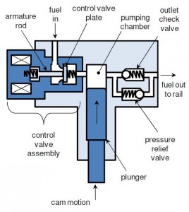
The fuel rail pressure in a GDI engine is provided by a cam-driven variable stroke high pressure fuel pump. In typical designs, the volume of fuel pumped is controlled by a Flow Control Valve (FCV) located on the inlet of the pump. The valve is electronically controlled by the engine control unit to regulate fuel rail pressure. The operation of the FCV is unique because its control must be synchronous with the crankshaft position.  Typical GDI fuel pumps have three lobes per camshaft revolution that stroke the pump.  Fuel pressure is regulated by controlling the FCV during the stroke of the pump to regulate how much of the stroke is allowed to draw fuel into the pumping chamber.

Fuel enters the pumping chamber during the downward motion of the plunger through the open FCV.  The FCV opens during this time due to the valve being held open by the spring and the suction of the piston.  This results in a lower pressure in the pumping chamber as compared to the fuel inlet, and fuel flows into the chamber.

If the FCV solenoid remains de-energized during the upward stroke of the cam and plunger, the valve stays open due to the spring force, preventing the pump from developing pressure.  The GDI fuel pump thus delivers no fuel to the fuel rail.

If the FCV solenoid is energized during the upward stroke, the FCV closes and the low pressure inlet is sealed off from the pumping chamber.  This allows high pressure to be developed in the chamber.  Once enough pressure has been developed, the outlet check valve opens and pressurized fuel is delivered to the fuel rail.

The quantity of fuel delivered by the GDI fuel pump can be adjusted by controlling the exact moment in the upward plunger stroke that the FCV solenoid is energized. The earlier the valve closes, the higher the quantity of fuel delivered to the fuel rail.

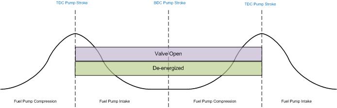
Fig 1: Zero Fuel Pressure

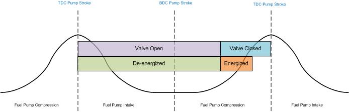
Fig 2: Mid-range Fuel Pressure

 

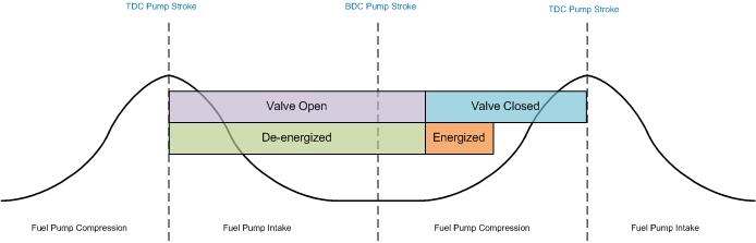
Fig 3: Maximum Fuel Pressure

Typically, a relief path using a pressure relief valve is also present to prevent over-pressurization of the fuel rail. This relief path is not normally used for fuel pressure control. The relief pressure setting is set higher than the maximum pressure expected during normal engine operation.  Operating the relief valve in this manner results in higher engine efficiency through reduced fuel pump drive losses. For example, during a deceleration fuel cut, no fuel will flow out of the fuel rail because the injectors are disabled. In such a case, the FCV solenoid can be left de-energized and the rail pressure will remain at its previous set point without the fuel pump adding any additional fuel, thus saving pumping work.

GDI Fuel Pump Control Algorithm

To create a closed loop pressure control algorithm using an angularly driven GDI fuel pump we start with developing a traditional feedforward and feedback control loop.  Determination of the fuel rail pressure target is not covered here, but traditionally it is based upon engine speed and torque demand.

Dana uses model based controls implemented using the Simulink development environment and the OpenECU blockset to create all the control commands necessary for use with a GDI pump. The control algorithm implements the fuel rail pressure target, and performs closed loop control of the fuel pressure.

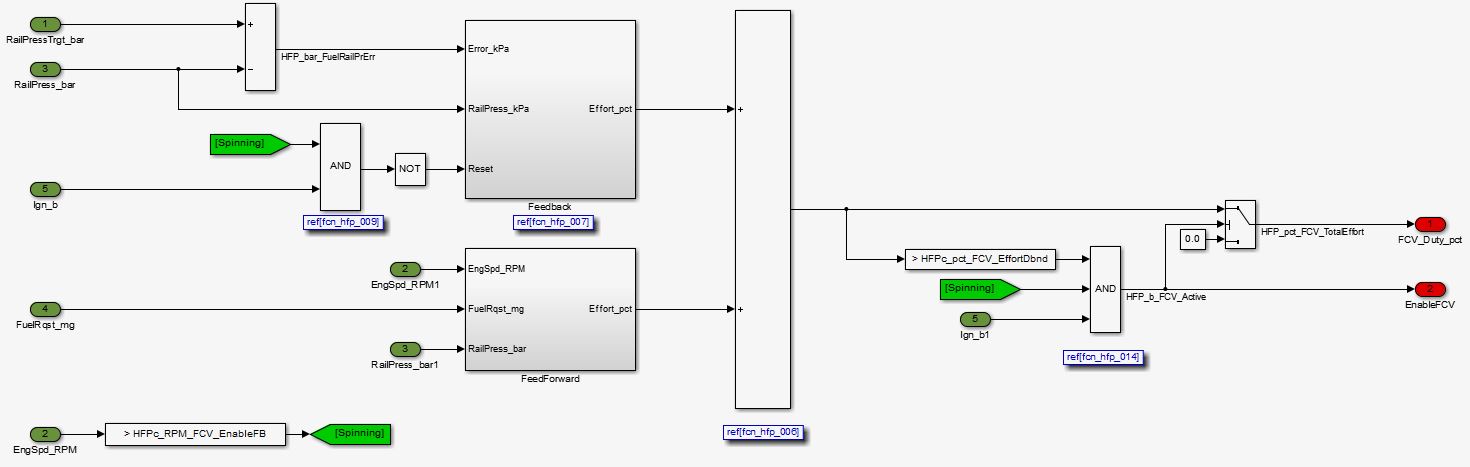
Fig 4: Feedforward & Feedback Control

If the actual fuel rail pressure is below the target, then the control effort is translated into a start of current angle for the FCV solenoid. This angle is specified relative to the TDC position of the fuel pump plunger. The higher the effort required, the earlier will be the ‘on-angle’ of the FCV solenoid. This transformation from effort to angular control is fully calibratable and can be characterized for different fuel pumps.

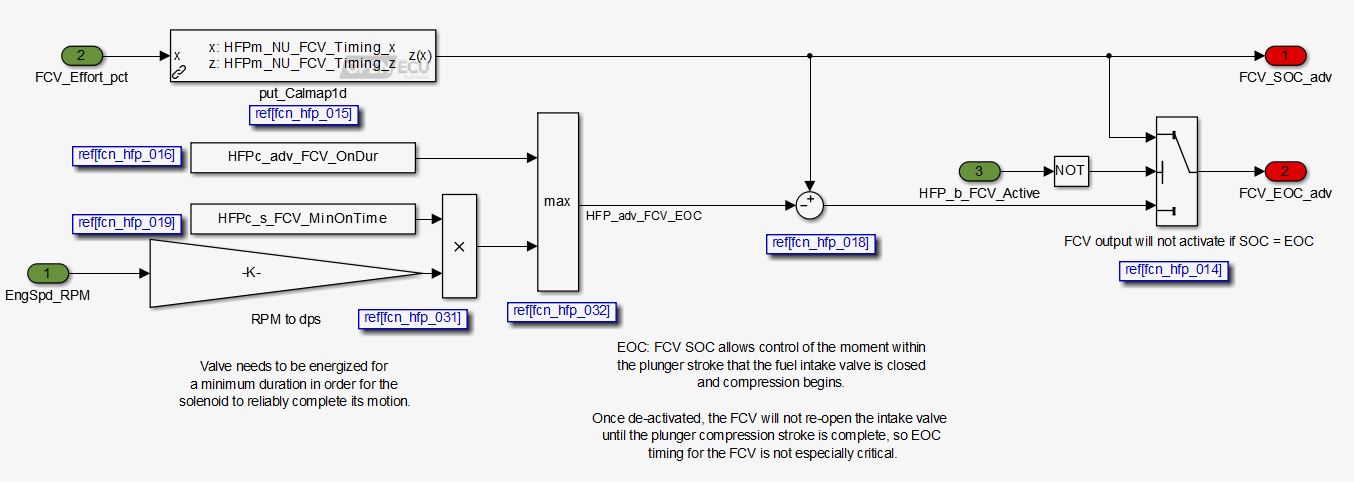
Fig 5: FCV Angular control

The duration for which the FCV is to be energized is also calculated based on engine speed and the target effort. The duration is not a critical parameter in GDI pump control. The FCV solenoid must be energized long enough so that enough pressure is developed in the pumping chamber to prevent the FCV from opening till the plunger begins its downward stroke.  By relying on the pressure in the pumping chamber to keep the FCV closed the on-time of the FCV circuit can be reduced which reduces current draw from the ECU and limits the heating of the ECU.

The ‘on-angle’ and duration are the used to calculate the ‘off-angle’ for the FCV solenoid, and these are fed to the OpenECU Simulink block.  The OpenECU driver software will schedule the angular tasks such that the FCV is energized and de-energized at the desired crankshaft positions.